Kumaraswamy custom brms family

Update: We finally published bayesfam, a package that contains a bunch of custom families for brms.

I am currently working with different unit interval distributions and one of the more common ones to be mentioned in the literature is the Kumaraswamy distribution Kumaraswamy (1980). As I am working with brms and there is no built-in family for the kumaraswamy distribution, I had to write a custom family for it. This blog post is a documentation of my process and could serve as a kind of tutorial I guess. I am roughly following the brms custom family vignette here, in case you want to take a look at it.

Before any code, let’s collect all the necessary information about the Kumaraswamy distribution. I took these from Mitnik (2013).

The probability density function for the unit interval is given as:

Now in brms I would like to have a mean parametrization for that density. Sadly, the mean is given by:

where $B$ is the beta function, which can not be inverted to solve for p or q. However, the quantile function is available in closed-form:

The median can be derived from the quantile function and results in a formula that can be solved for q:

Median Parametrization

library(brms)

To build the median parametrization I first wrote a function for the given pdf and then replaced each occurrence of q with the result from the last section. While there is room to improve, this is just a first draft.

median_dkumaraswamy <- function(x, md, p) {
  p *
    (-(log(2) / log(1 - md^p))) *
    x^(p - 1) *
    (1 - x^p)^((-(log(2) / log(1 - md^p))) - 1)
}

Let’s see if the density looks as it should with a symmetric, an asymmetric and a bathtub shape.

x = seq(from = 0, to = 1, length.out = 10000)[2:9999] # exclude 0 and 1

layout(matrix(1:3, ncol = 3))
plot(
  x,
  median_dkumaraswamy(x, md = 0.5, p = 4),
  type = "l",
  ylab = "Density",
  main = "Symmetric Kumaraswamy"
)
plot(
  x,
  median_dkumaraswamy(x, md = 0.75, p = 4),
  type = "l",
  ylab = "Density",
  main = "Asymmetric Kumaraswamy"
)
plot(
  x,
  median_dkumaraswamy(x, md = 0.5, p = 0.25),
  type = "l",
  ylab = "Density",
  main = "Bathtub Kumaraswamy"
)

And while this might not be possible for every distribution, chances are high that someone else already wrote a density you could check against. In the case of the kumaraswamy distribution, I was lucky.

layout(matrix(1:3, ncol = 3))
plot(
  x,
  median_dkumaraswamy(x, 0.5, 4) -
    extraDistr::dkumar(x, 4, -log(2) / log(1 - 0.5^4)),
  ylab = "Difference",
  main = "Symmetric: Mine - extraDistr"
)
plot(
  x,
  median_dkumaraswamy(x, 0.75, 4) -
    extraDistr::dkumar(x, 4, -log(2) / log(1 - 0.75^4)),
  ylab = "Difference",
  main = "Asymmetric: Mine - extraDistr"
)
plot(
  x,
  median_dkumaraswamy(x, 0.5, 0.25) -
    extraDistr::dkumar(x, 0.25, -log(2) / log(1 - 0.5^0.25)),
  ylab = "Difference",
  main = "Bathtub: Mine - extraDistr"
)

And it seems as if all is well here.

Now you might be asking why I would want to write my own density function if there already was one. The answer is that I have to write stan code for the log-pdf for the custom family and before I do that, I want to have a working version in R that I can test. And all this is also an exercise in case I need to write one of these without a preexisting implementation.

Log-Density-Function

While writing my own proper density function, I have to keep in mind, that stan uses the log-pdf as it is a lot more numerically robust, so I shall do the same for the R version of my code.

To make this work well, I can’t just wrap the density function in a log Instead, I have to use the rules for logarithms like $log(x^r) = rlog(x)$ and composite functions like log1p to get the most out of the transformation. In case I’d want the density on the natural scale, I just throw an exp on the result. Add some input checks and the results looks like this:

# Density function (median parametrization)
dkumaraswamy <- function(x, mu, p, log = FALSE) {
  if (isTRUE(any(x <= 0 | x >= 1))) {
    stop("x must be in (0,1).")
  }
  if (isTRUE(any(mu < 0 | mu > 1))) {
    stop("The mean must be in (0,1).")
  }
  mu[which(mu > 0.999999)] <- 0.999999
  mu[which(mu < 0.000001)] <- 0.000001
  if (isTRUE(any(p <= 0))) {
    stop("P must be above 0.")
  }
  logpdf <- log(p) +
    log(log(2)) -
    log(-(log1p(-mu^p))) +
    (p - 1) * log(x) +
    ((-(log(2) / log1p(-mu^p))) - 1) * log1p(-x^p)

  if (log) {
    return(logpdf)
  } else {
    return(exp(logpdf))
  }
}

I compare this to the implementation from earlier to test for implementation problems again and can see that the differences are on the float resolution scale, which is what I would expect as the difference between just wrapping in log() and further optimizing the code.

layout(matrix(1:3, ncol = 3))

md = 0.5
p = 4
plot(
  log(median_dkumaraswamy(x, md, p)) - dkumaraswamy(x, md, p, log = TRUE),
  ylab = "Difference",
  main = "Symmetric: Simple log - Advanced log"
)

md = 0.75
plot(
  log(median_dkumaraswamy(x, md, p)) - dkumaraswamy(x, md, p, log = TRUE),
  ylab = "Difference",
  main = "Asymmetric: Simple log - Advanced log"
)

md = 0.5
p = 0.25
plot(
  log(median_dkumaraswamy(x, md, p)) - dkumaraswamy(x, md, p, log = TRUE),
  ylab = "Difference",
  main = "Bathtub: Simple log - Advanced log"
)

RNG

Now, while this is not necessary to fit models with the kumaraswamy distribution, I needed an rng anyways, so I figured, I could just add the code here for a quick showcase of the inverse cdf method of building an rng. The inverse cdf method uses the fact that there is simple quantile- or cumulative density function that can be used to transform a uniform random variable to a kumaraswamy distributed one. As a reminder, that is the same function we used to derive the median, which is simply the 50th percentile. Essentially we randomly point at a quantile and ask the quantile function, what number it corresponds to.

# Random generation (median parametrization)
rkumaraswamy <- function(n, mu = 0.5, p = 2) {
  if (isTRUE(any(mu <= 0 | mu >= 1))) {
    stop("The mean must be in (0,1).")
  }
  mu[which(mu > 0.999999)] <- 0.999999
  mu[which(mu < 0.000001)] <- 0.000001
  if (isTRUE(any(p <= 0))) {
    stop("P must be above 0.")
  }
  q <- -(log(2) / log1p(-mu^p))
  return(
    (1 - (1 - runif(n, min = 0, max = 1))^(1 / q))^(1 / p)
  )
}

To test the RNG, I generate three samples, as before, and see if it recovers the median and passes a visual check to match the form I would expect.

layout(matrix(1:3, ncol = 3))
y = rkumaraswamy(10000, mu = 0.5, p = 4)
hist(y, main = paste("Median:", median(y)))

y = rkumaraswamy(10000, mu = 0.75, p = 4)
hist(y, main = paste("Median:", median(y)))

y = rkumaraswamy(10000, mu = 0.5, p = 0.25)
hist(y, main = paste("Median:", median(y)))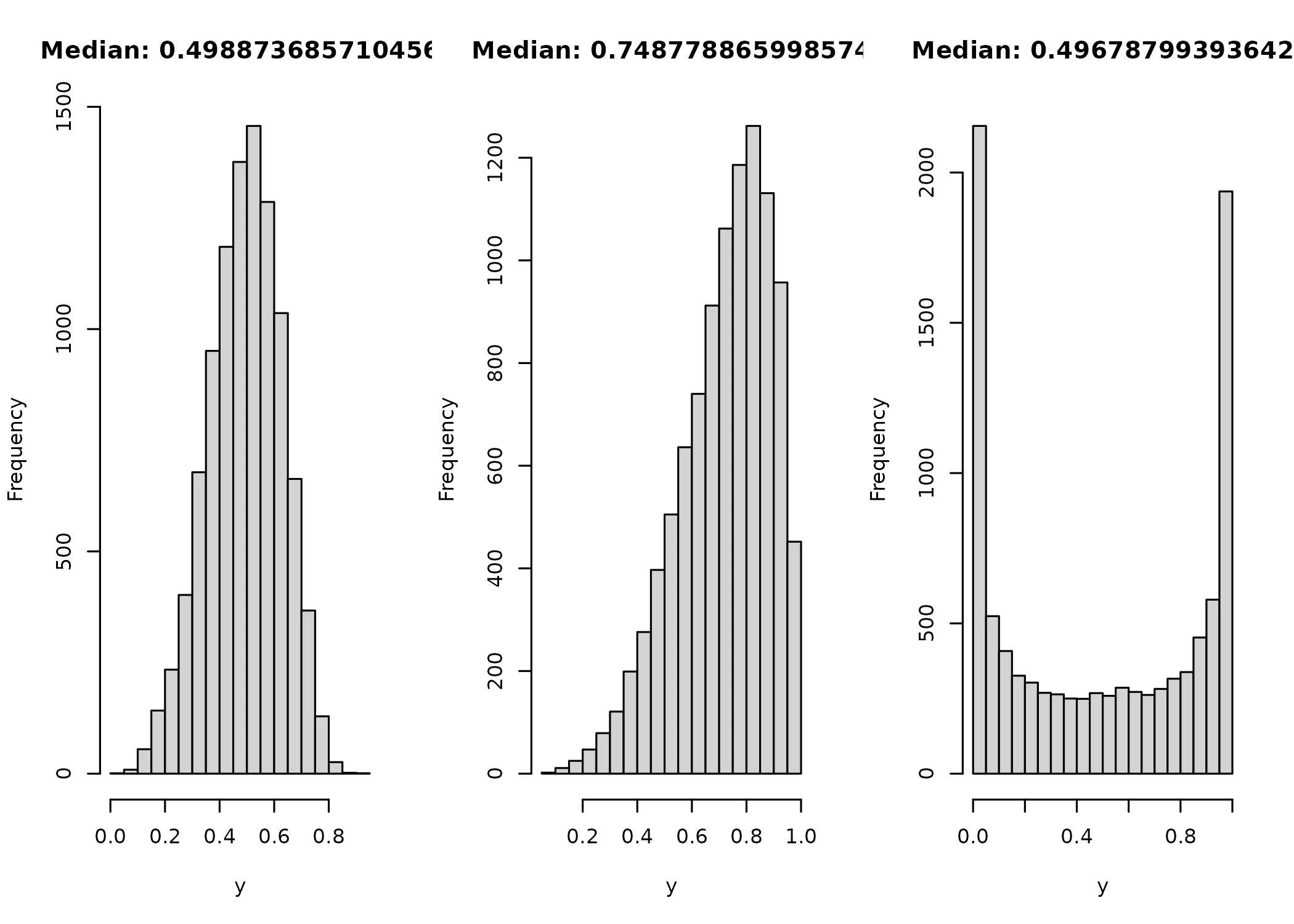

In all three cases, both the distribution and median look like I’d like them to.

Post-Processing

Before I can start writing the complete family, I also want to add support for all the cool post-processing things brms supports, like calculating the log likelihood of an observation, as needed for elpd based loo calculations. This can be built from the log pdf, the posterior samples and observation provided by brms.

log_lik_kumaraswamy <- function(i, prep) {
  mu <- get_dpar(prep, "mu", i = i)
  p <- get_dpar(prep, "p", i = i)
  y <- prep$data$Y[i]
  return(dkumaraswamy(y, mu, p, log = TRUE))
}

The second post-processing step I’d like to support is the posterior_predict function, as used by posterior predictive plots for rough model misspecification. Here I just generate random numbers using the parameters provided by brms.

posterior_predict_kumaraswamy <- function(i, prep, ...) {
  mu <- get_dpar(prep, "mu", i = i)
  p <- get_dpar(prep, "p", i = i)
  return(rkumaraswamy(prep$ndraws, mu, p))
}

The last step of post processing that is part of the custom family vignette is the posterior_epred function, used for example for conditional effects. This requires the calculation of the posterior mean. Luckily I already have an equation for the mean, so I can just recover q as done in the intro and plug p and q into the equation for the mean. All done again with the parameters supplied by brms.

posterior_epred_kumaraswamy <- function(prep) {
  mu <- get_dpar(prep, "mu")
  p <- get_dpar(prep, "p")
  q <- -(log(2) / log1p(-mu^p))
  return(q * beta((1 + 1 / p), q))
}

Custom brms Family

And with all that out of the way, it is time to built the actual custom family. I wrapped the custom_family call so I could set the link function that I wanted and add the stanvars to the family object, to make it self contained.

The stanvars contain the stan code for the lpdf and rng, which is mostly a simple copy of the R code with some small adjustments when built in functions of R and stan differ, such as the use of log1m(x) in stan instead of log1p(-x) in R.

The rest of the function is naming of the parameters, setting links on them, defining lower and upper bounds, the scale of the distribution and adding the post processing functions from above.

kumaraswamy <- function(link = "logit", link_p = "log") {
  family <- custom_family(
    "kumaraswamy",
    dpars = c("mu", "p"),
    links = c(link, link_p),
    lb = c(0, 0),
    ub = c(1, NA),
    type = "real",
    log_lik = log_lik_kumaraswamy,
    posterior_predict = posterior_predict_kumaraswamy,
    posterior_epred = posterior_epred_kumaraswamy
  )
  family$stanvars <- stanvar(
    scode = "
      real kumaraswamy_lpdf(real y, real mu, real p) {
         return  (log(p) + log(log(2)) - log(-(log1m(mu^p))) + (p-1) * log(y) +
                 ((-(log(2)/log1m(mu^p)))-1) * log1m(y^p));
      }

      real kumaraswamy_rng(real mu, real p) {
         return ((1-(1-uniform_rng(0, 1))^(1/(-(log(2)/log1m(mu^p)))))^(1/p));
      }",
    block = "functions"
  )
  return(family)
}

And with that, the custom family is done.

brms fitting

Before leaving, I should obviously show you that it actually works. So here is a quick example where I generate a dataset, fit a kumaraswamy model to it and run some of the post processing I prepared for:

a = rnorm(1000)
data = list(a = a, y = rkumaraswamy(1000, inv_logit_scaled(0.2 + 0.5 * a), 4))
hist(data$y)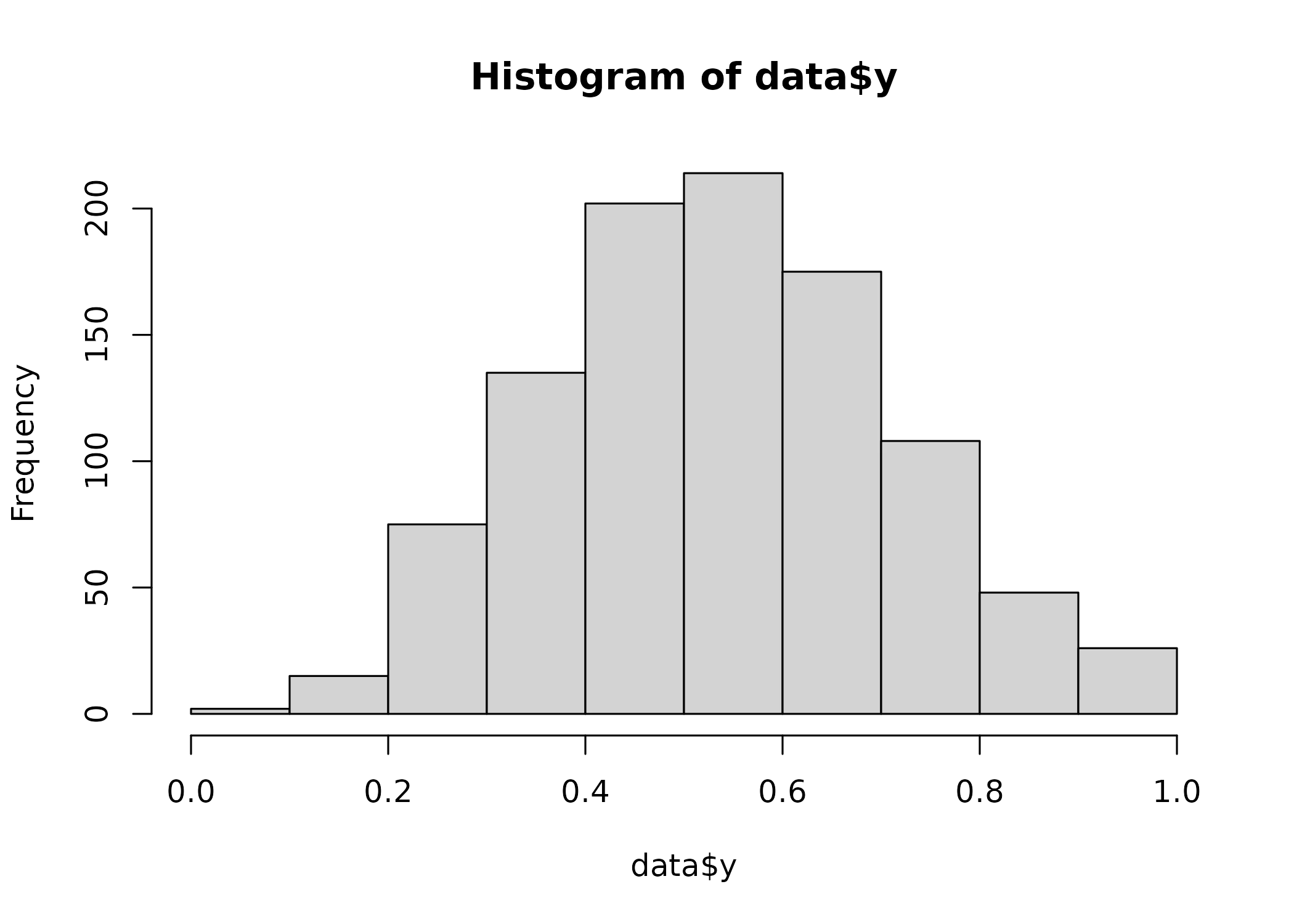

fit1 <- brm(
  y ~ 1 + a,
  data = data,
  family = kumaraswamy(),
  stanvars = kumaraswamy()$stanvars
)

 Family: kumaraswamy 
  Links: mu = logit 
Formula: y ~ 1 + a 
   Data: data (Number of observations: 1000) 
  Draws: 4 chains, each with iter = 2000; warmup = 1000; thin = 1;
         total post-warmup draws = 4000

Regression Coefficients:
          Estimate Est.Error l-95% CI u-95% CI Rhat Bulk_ESS Tail_ESS
Intercept     0.21      0.02     0.17     0.25 1.00     2250     2251
a             0.51      0.02     0.48     0.55 1.00     2738     2886

Further Distributional Parameters:
  Estimate Est.Error l-95% CI u-95% CI Rhat Bulk_ESS Tail_ESS
p     3.92      0.12     3.70     4.16 1.00     2465     2488

Draws were sampled using sampling(NUTS). For each parameter, Bulk_ESS
and Tail_ESS are effective sample size measures, and Rhat is the potential
scale reduction factor on split chains (at convergence, Rhat = 1).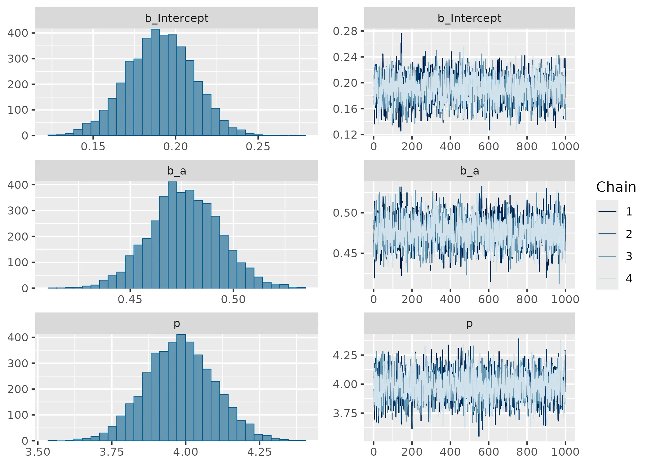

The summary shows that the model is sampling well and can recover the parameters. There are also no sampling problems to see in the Rhat, ESS and trace plot. Wonderfull. So how about a posterior predictive check anyone? Wouldn’t that be something?

pp_check(fit1)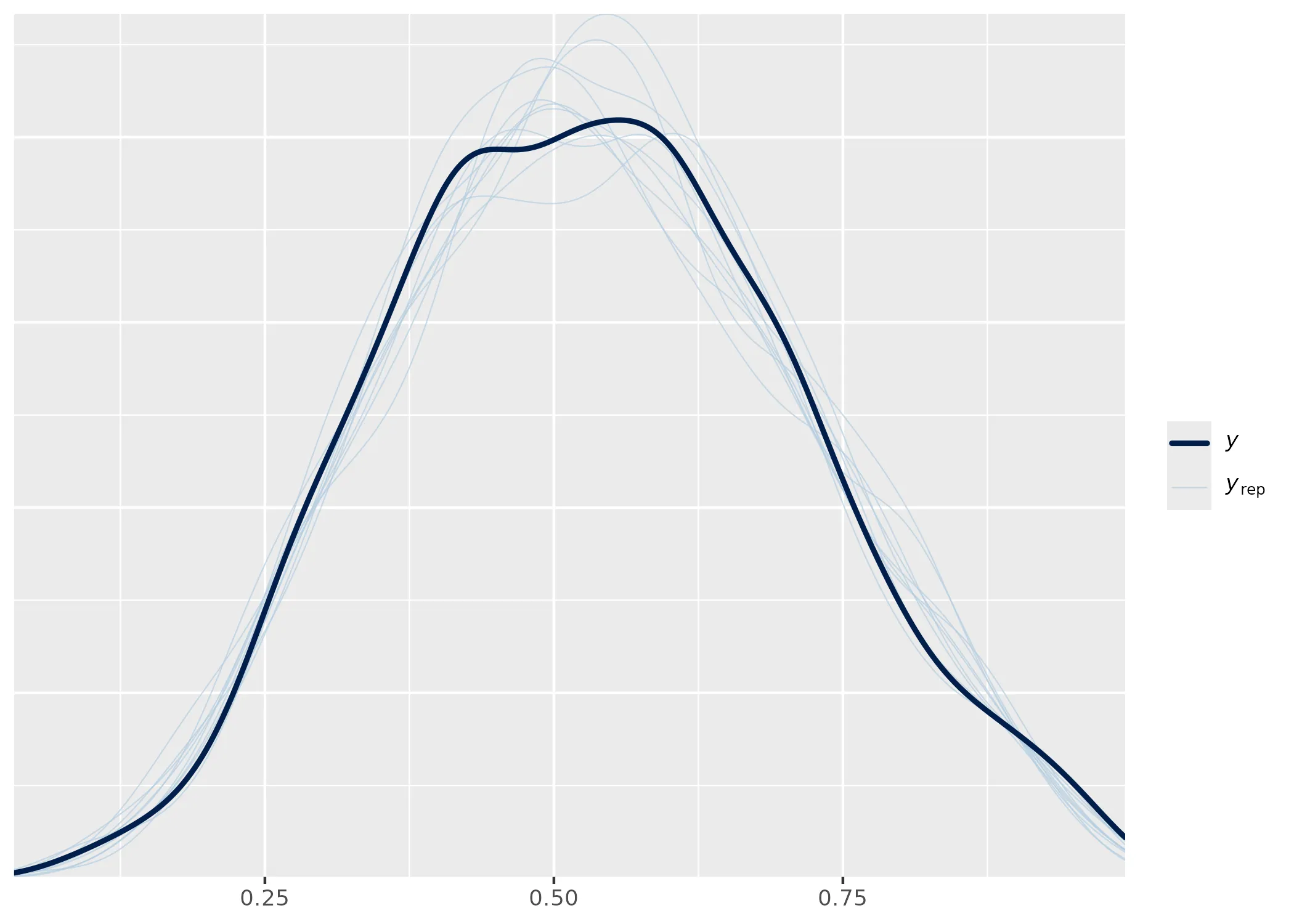

I would say that looks quite fine. But how about those conditional effects?

conditional_effects(fit1)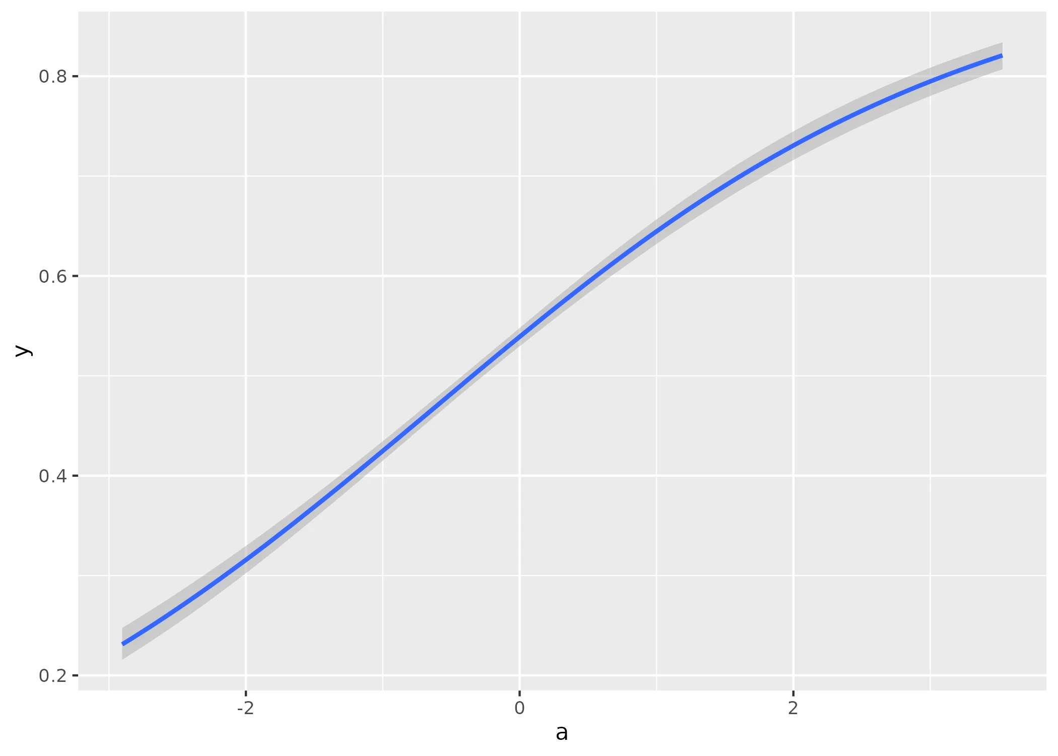

That also looks like I would expect it to.

Finally, lets calculate the loo-elpd for the fit and compare it to one using a beta likelihood:

loo_kumaraswamy <- loo::loo(fit1)
loo_kumaraswamy

Computed from 4000 by 1000 log-likelihood matrix.

         Estimate   SE
elpd_loo    581.2 19.9
p_loo         3.1  0.3
looic     -1162.3 39.8
------
MCSE of elpd_loo is 0.0.
MCSE and ESS estimates assume MCMC draws (r_eff in [0.5, 1.2]).

All Pareto k estimates are good (k < 0.7).
See help('pareto-k-diagnostic') for details.

fit2 <- brm(
  y ~ 1 + a,
  data = data,
  family = Beta()
)

     elpd_diff se_diff
fit1   0.0       0.0  
fit2 -31.0       8.5  

Nice. To nobodies surprise, the kumaraswamy fit had better predictive performance than the beta fit hehe.

And that’s it. At this point the custom family is ready to use and supports all the good things brms comes with.

Bibliography

Kumaraswamy, Ponnambalam. 1980. “A Generalized Probability Density Function for Double-Bounded Random Processes.” Journal of Hydrology 46 (1-2): 79–88.
Mitnik, Pablo A. 2013. “New Properties of the Kumaraswamy Distribution.” Communications in Statistics-Theory and Methods 42 (5): 741–55.